Download Weather Layers as Images and Data
List the available weather layers, then get radar precipitation rate as a ready-to-display PNG and model wind speed as a NetCDF file of raw values.
Oct 9, 2026 · Python
Weather layers are gridded products covering a whole area: radar precipitation rate, lightning density, hail size, and forecast model fields like temperature and wind. The layers endpoint returns any of them for a bounding box you choose, in one of two forms:
- a PNG image with the color scale already applied, ready to show on a map or a web page;
- a NetCDF file of the raw values, for analysis.
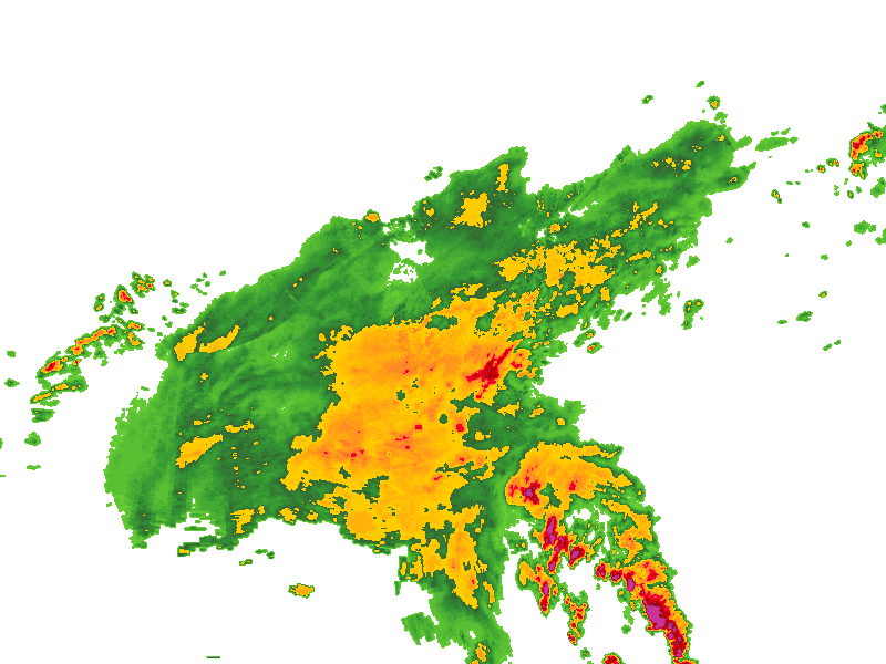
This tutorial finds a layer, downloads radar precipitation rate (2minMRMSPrecipRate) as a PNG, then downloads forecast wind speed (15minHRRRWindSpeed) as NetCDF.
You'll need a MyRadar API key and Python 3 with requests, xarray, netCDF4 and matplotlib (pip install requests xarray netCDF4 matplotlib).
1. List the available layers#
Every layer request needs a layer name, and /layers/listlayers is where the names come from. It takes no parameters and returns a JSON array of strings, one per layer:
import requests

MYRADAR_API_KEY = "YOUR_KEY"
headers = {"Subscription-Key": MYRADAR_API_KEY}
BASE = "https://api.myradar.dev/v1/layers"

response = requests.get(f"{BASE}/listlayers", headers=headers)
response.raise_for_status()
layers = response.json()
print(len(layers), "layers")
There are over 90 layers, and the list grows, so call the endpoint rather than copying names from anywhere else, this page included.
Most names follow one pattern: how often the layer updates, then where the data comes from, then what it measures. 2minMRMSPrecipRate is a new precipitation rate every 2 minutes from MRMS, the multi-radar, multi-sensor radar analysis. 15minHRRRWindSpeed is wind speed every 15 minutes from HRRR, NOAA's High-Resolution Rapid Refresh forecast model. Some names add a prefix such as Latest, Lagged, Forecast or Delta for a variant of a layer.
The layers fall into a few families:
| Family | Example layers |
|---|---|
| Radar (MRMS) | 2minMRMSPrecipRate, 15minMRMSPrecipRate, 1hrMRMSPrecipRate, 15minMRMSPrecipType |
| Hail | 2minMaxEstimatedSizeHail, 2minSevereHailProbability, DailyHailSwath |
| Lightning | 5minAvgDensityLightningStrikes, 30minLightningProbability |
| Nowcast | NowcastPrecipRate, 1minNowcastReflectivity |
| Forecast model, US (HRRR) | 15minHRRRWindSpeed, 15minHRRRAirTemperature, Forecast15minHRRRPrecipRate, 1hrHRRRCloudCover |
| Forecast model, global (GFS) | GFSWindSpeed, GFSTemp, GFSPrecipRate |
| Roads | 15minRoadCondition, 15minHRRRRoadTemperature |
Because the names follow a pattern, you can filter the list in code. For example, every radar layer, or every wind speed layer:
radar = [name for name in layers if "MRMS" in name]
wind = [name for name in layers if "WindSpeed" in name]
print(radar)
print(wind)
Check a name is in the list before you use it: a name that isn't, including a misspelling, fails with a 400.
2. Get the layer's time step and color scale#
Before requesting a layer, look it up with /layers/layerinfo/{layer}. It tells you the two things every layer request depends on: the layer's time step, which decides the valid times you can ask for, and its color scale, which is how the PNG is colored:
info = requests.get(f"{BASE}/layerinfo/2minMRMSPrecipRate", headers=headers).json()
print("New data every", info["time_step"], "seconds") # 120 for this layer| Field | Meaning |
|---|---|
time_step | Seconds between valid times. Step 3 uses it to pick a valid time. |
levels | The values the color scale changes at, in the layer's units. |
colors | One color per level, in the same order, as RGBA values from 0 to 1: four numbers per color. |
labels | Text labels for the levels, where a layer has them. |
Time steps differ by layer, so look up each layer you use rather than reusing one layer's value for another.
The color scale is what you need for a legend beside the PNG. Group colors into fours and pair each color with its level:
import matplotlib.pyplot as plt

colors = info["colors"]
rgba = [tuple(colors[i:i + 4]) for i in range(0, len(colors), 4)]
levels = info["levels"]

fig, ax = plt.subplots(figsize=(7, 0.9))
ax.bar(range(len(levels)), [1] * len(levels), width=1, color=rgba)
ax.set_xlim(-0.5, len(levels) - 0.5)

every = max(1, len(levels) // 8)  # label about eight levels so the numbers stay readable
ticks = range(0, len(levels), every)
ax.set_xticks(ticks, [f"{levels[i]:.3g}" for i in ticks])
ax.set_yticks([])
for side in ax.spines.values():
    side.set_visible(False)
ax.set_title("2minMRMSPrecipRate color scale", loc="left")
plt.show()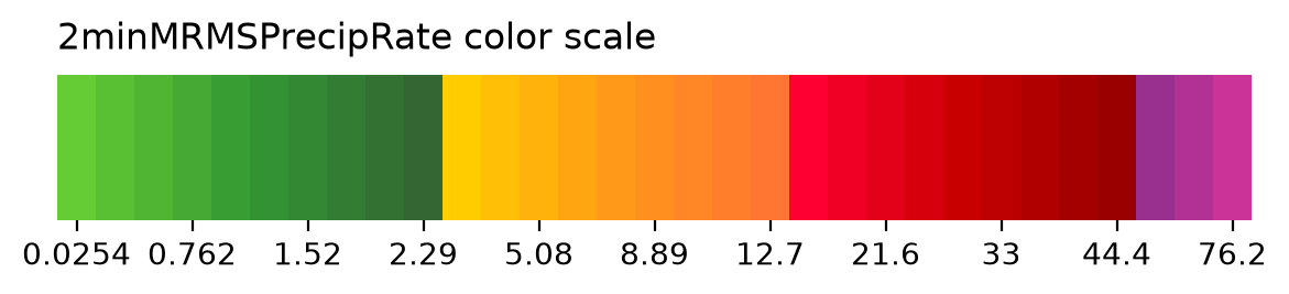
This layer's levels are in millimeters per hour. The NetCDF download in step 5 tells you any layer's units.
3. Pick a valid time#
Every request names the time you want, its valid time, as YYYYmmdd.HHMM in UTC. Layer data is available both historically and in real time, so the valid time can be in the past or, for forecast layers, the future:
| Kind of layer | Examples | Valid times you can ask for |
|---|---|---|
| Observations | radar (MRMS), hail, lightning | The past, up to close to the current time. Radar runs about 4 to 5 minutes behind real time, and a time further ahead than the newest scan returns 404. |
| Forecast model | HRRR, GFS | The past, and the future: a future valid time returns the model's forecast for that time. |
Whatever the time, it has to line up with the layer's time step. This helper rounds any time down to a multiple of time_step and formats it:
from datetime import datetime, timedelta, timezone

def valid_time(when, time_step):
    """`when` rounded down to the layer's time step, as YYYYmmdd.HHMM in UTC."""
    t = when.timestamp() // time_step * time_step
    return datetime.fromtimestamp(t, timezone.utc).strftime("%Y%m%d.%H%M")

now = datetime.now(timezone.utc)

# Radar, as close to now as it's available: step back a few minutes for processing
recent = valid_time(now - timedelta(minutes=5), info["time_step"])

# Any past time, for history: a storm on 21 May 2024 at 20:20 UTC
past = valid_time(datetime(2024, 5, 21, 20, 20, tzinfo=timezone.utc), info["time_step"])
If a request for the newest time returns 404, the data isn't ready yet: step back one more time step. For forecast layers you'll pass a time in the future instead, as step 5 does.
4. Download precipitation rate as a PNG#
The area and image size go in the path: the upper-left corner, the lower-right corner, then the width and height in pixels. This requests an 800 × 600 image of the northeastern Gulf of Mexico:
ul_lat, ul_lon, lr_lat, lr_lon = 32.5, -90.5, 26.5, -80.5
width, height = 800, 600

url = (f"{BASE}/layer/2minMRMSPrecipRate/{recent}"
       f"/{ul_lat}/{ul_lon}/{lr_lat}/{lr_lon}/{width}/{height}")
response = requests.get(url, headers=headers)
response.raise_for_status()

with open("precip_rate.png", "wb") as f:
    f.write(response.content)
print("Saved", recent, response.headers["Content-Type"])  # image/png
The image at the top of this page is one of these downloads. It's colored with the layer's color scale from step 2, so the legend you built there matches it, and it's transparent wherever no precipitation is falling, so it sits cleanly on top of a map. It's drawn in Web Mercator (epsg=3857 by default), the projection web maps use, so you can place it on a Mapbox, Leaflet or Google map as an image overlay over the same bounding box.
5. Download wind speed as NetCDF#
To get the raw values instead of a picture, ask for NetCDF and turn the color scale off: as_netcdf=true together with apply_color=false. With as_netcdf=true alone, the color scale still applies and you get a PNG back.
Wind speed comes from the HRRR forecast model, so the valid time can be in the future: this asks for the forecast three hours from now, on the wind layer's own 15-minute time step:
import matplotlib.pyplot as plt
import xarray as xr

wind_info = requests.get(f"{BASE}/layerinfo/15minHRRRWindSpeed", headers=headers).json()
forecast_time = valid_time(now + timedelta(hours=3), wind_info["time_step"])

url = (f"{BASE}/layer/15minHRRRWindSpeed/{forecast_time}"
       f"/{ul_lat}/{ul_lon}/{lr_lat}/{lr_lon}/{width}/{height}")
params = {"as_netcdf": "true", "apply_color": "false"}
response = requests.get(url, headers=headers, params=params)
response.raise_for_status()

with open("wind_speed.nc", "wb") as f:
    f.write(response.content)
The file holds one grid of values plus everything needed to interpret it:
| Variable | What it holds |
|---|---|
var_data | The values: one per pixel, height rows by width columns, north at the top. |
units | The values' units as text, such as m/s for wind speed or mm/hr for precipitation rate. |
geo | Where the grid sits: [west, x step, 0, north, 0, y step] in degrees, the bounding box divided by the image size. |
epsg | The grid's projection, 3857 (Web Mercator) unless you asked for another. |
levels, colors | The layer's color scale, the same as in its layer info. |
Read the values, their units and the grid's position:
ds = xr.open_dataset("wind_speed.nc")

wind = ds["var_data"]            # one value per pixel, rows from north to south
units = str(ds["units"].values)  # "m/s" for wind speed
west, x_step, _, north, _, y_step = ds["geo"].values

print(wind.shape, units)
print(f"{float(wind.min()):.1f} to {float(wind.max()):.1f} {units}")
Then plot it, placing the grid with the corners from geo:
rows, cols = wind.shape
extent = [west, west + x_step * cols, north + y_step * rows, north]

plt.imshow(wind, extent=extent, cmap="Blues")
plt.colorbar(label=f"Wind speed ({units})", shrink=0.75)
plt.title(f"Forecast wind speed, {forecast_time} UTC")
plt.show()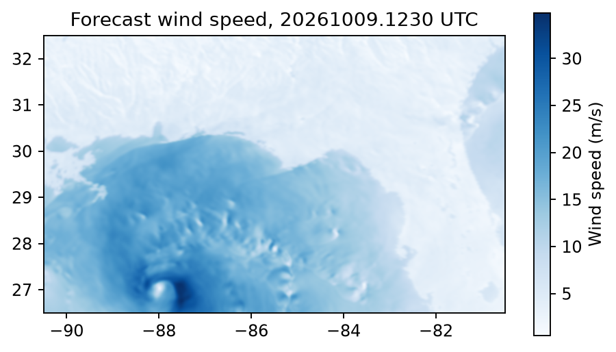
This forecast shows a tropical cyclone in the eastern Gulf, with the calm of its eye surrounded by the strongest winds. From here wind is an ordinary xarray array: pick out values by row and column, compute statistics, or save it in another format.
Layer endpoint reference#
GET /layers/layer/{layer}/{valid_time}/{ul_lat}/{ul_lon}/{lr_lat}/{lr_lon}/{width}/{height}
| Parameter | Default | What it does |
|---|---|---|
apply_color | true | Color the image with the layer's color scale. Set to false for raw values. |
as_netcdf | false | Return a NetCDF file of raw values. Needs apply_color=false. |
as_csv | false | Return the values as CSV. |
as_json | false | Return the values as JSON. |
epsg | 3857 | Projection of the output, as an EPSG code. |
A 400 means a parameter is invalid, such as a layer name that doesn't exist, and a 404 means there's no data for that valid time.
Next steps#
- To animate a layer as a GIF over a map, see Make a weather animation with gifbox.
- To read a layer at specific points instead of a whole area, use
/layers/point/{layer}/{valid_time}with alatlonslist. - To show a layer on an interactive map, use
/layers/tile/..., which returns standard x/y/z map tiles.